Step by step process of Creating a Pivot Table for a sheet of Data NOTE: To use this Skill User need to Login into Microsoft Applications
-
1.
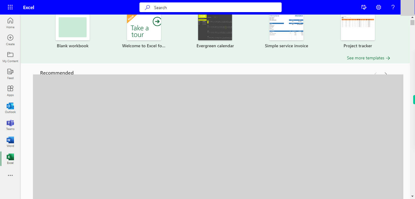
Open Microsoft Excel on the Web.
-
2.
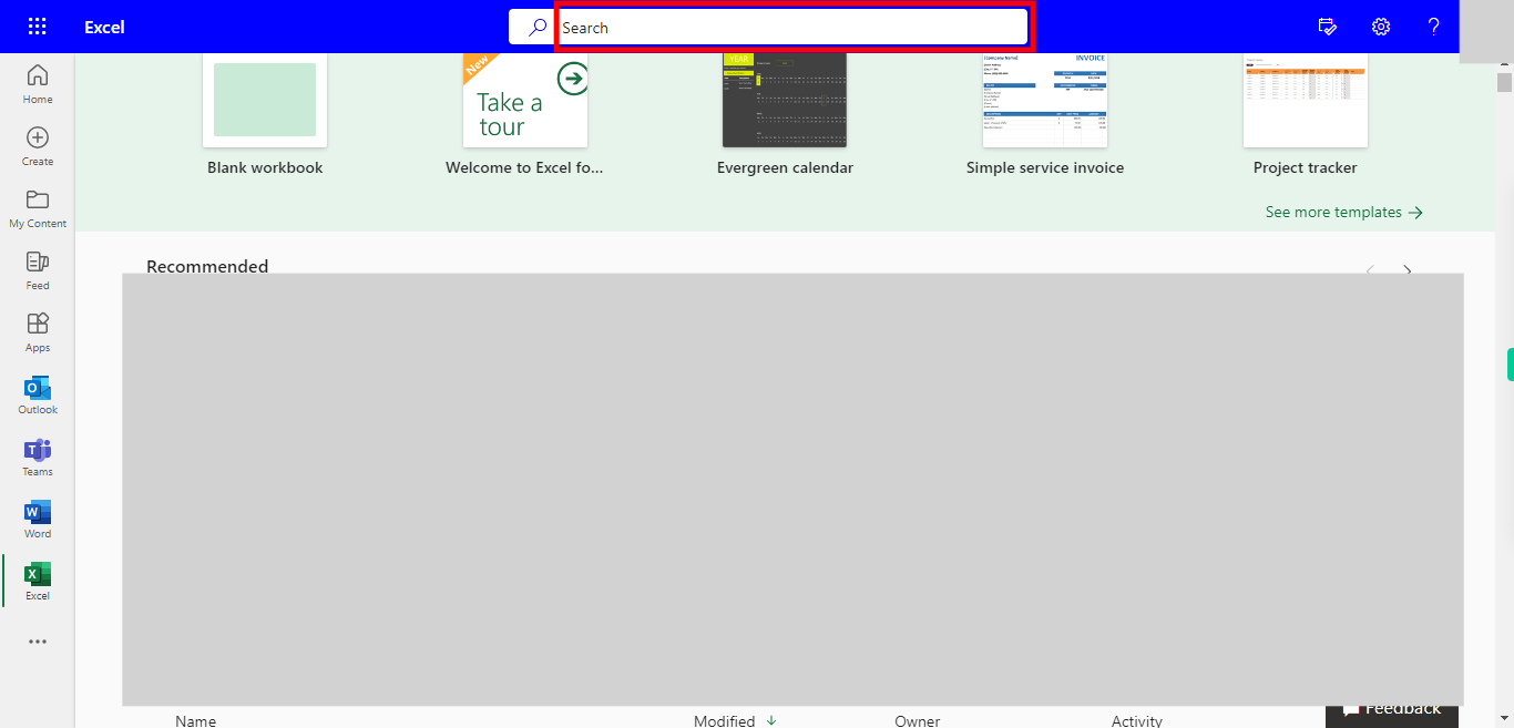
Click on Search Bar, Which enables the User to find the files in Outlook Excel. Type the file name, which will show recently Opened files. Once done, click on the "Next" button on the Supervity instruction widget. Open the File under the Search bar.
-
3.
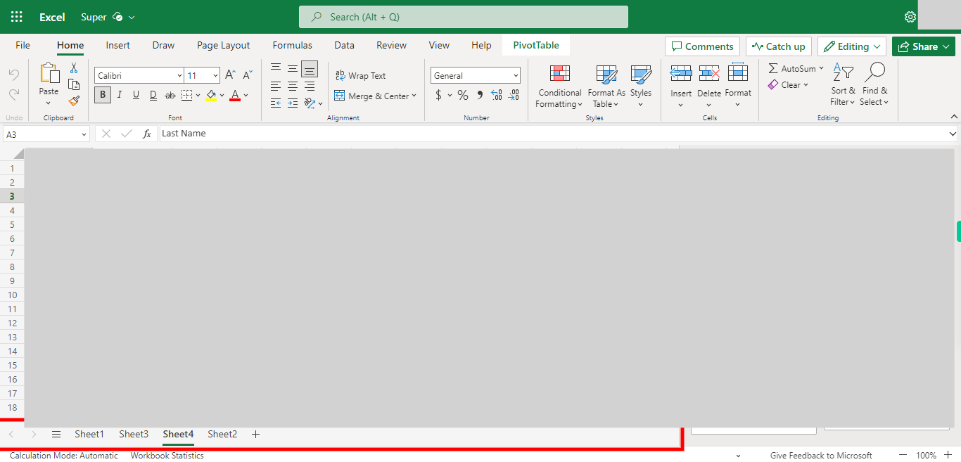
Go to the Sheet Where you want to Add a Pivot Table. Once done, click on the "Next" button on the Supervity instruction widget.
-
4.
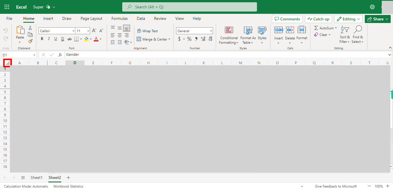
Click on Arrow Button to Select the Whole Data in the Sheet.
-
5.
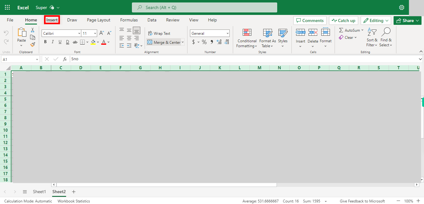
Click on Insert Tab.
-
6.
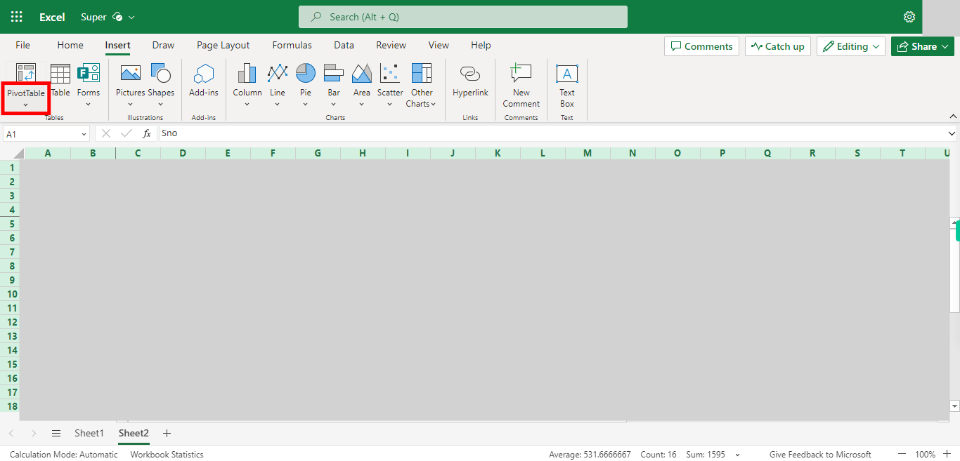
Click on the PivotTable drop-down.
-
7.
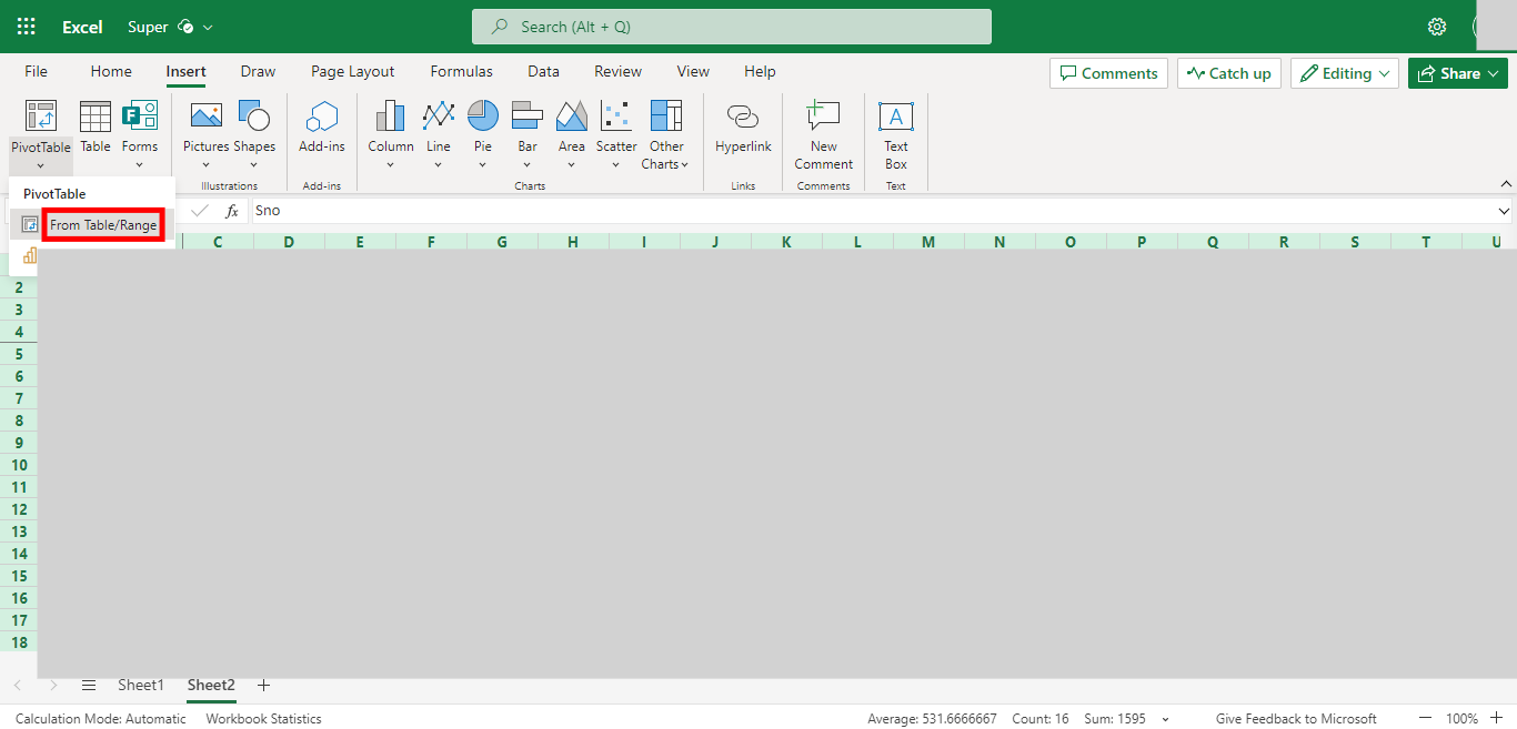
Click on From Table/Range
-
8.
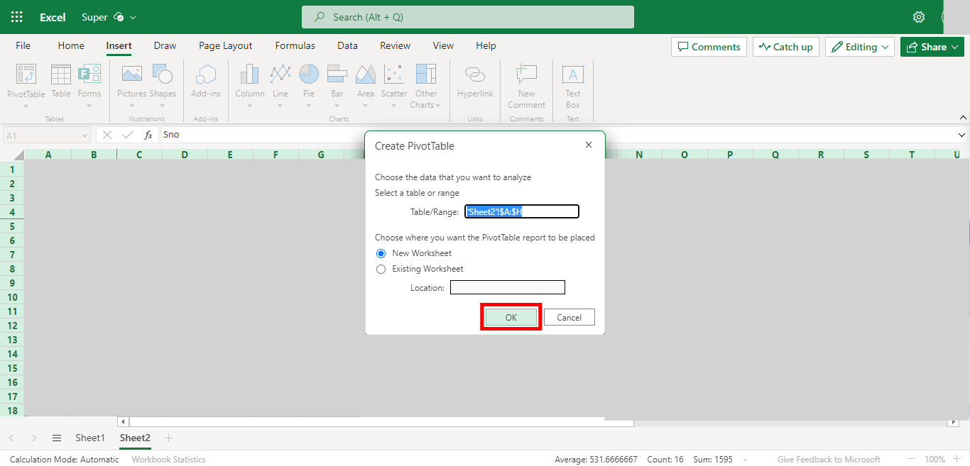
Click on OK
-
9.
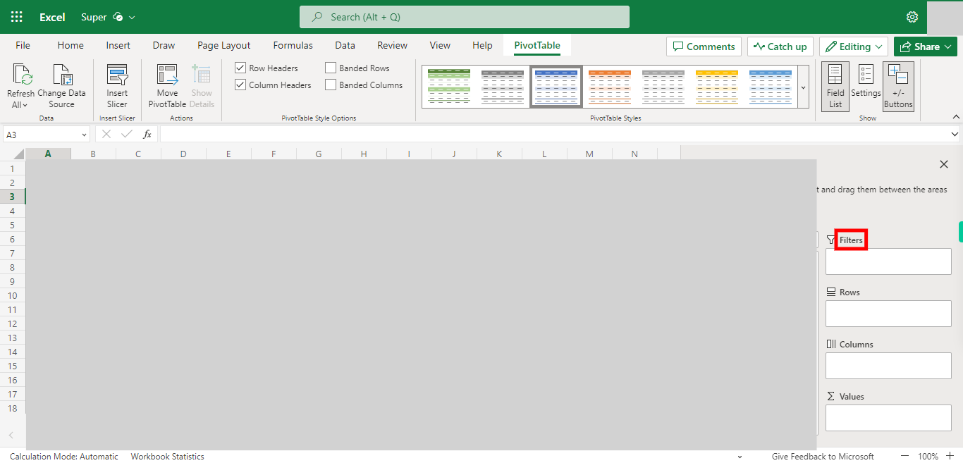
Drag and Drop the Columns You want to add into Filters. Once done, click on the "Next" button on the Supervity instruction widget.
-
10.
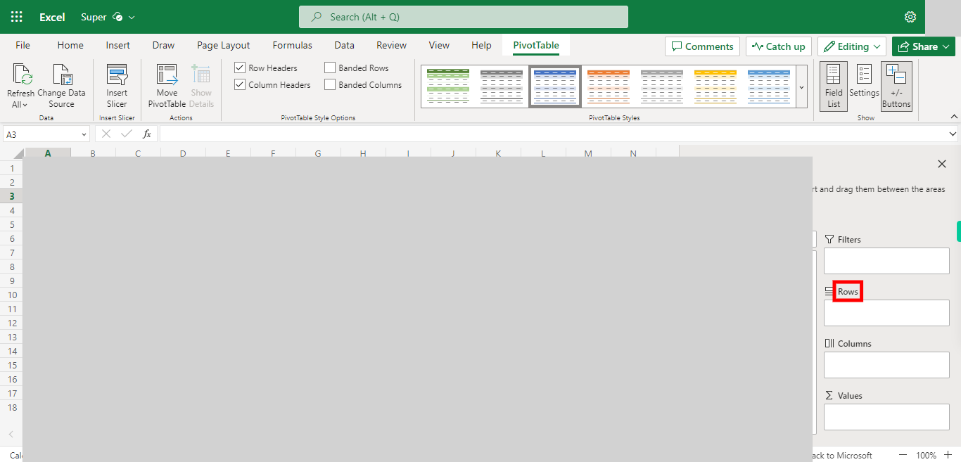
Drag and Drop Row data values from the list of Columns. Once done, click on the "Next" button on the Supervity instruction widget.
-
11.
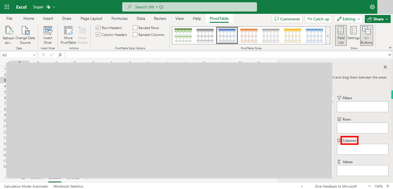
Drag and Drop the Column data values from the list of Columns. Once done, click on the "Next" button on the Supervity instruction widget.
-
12.
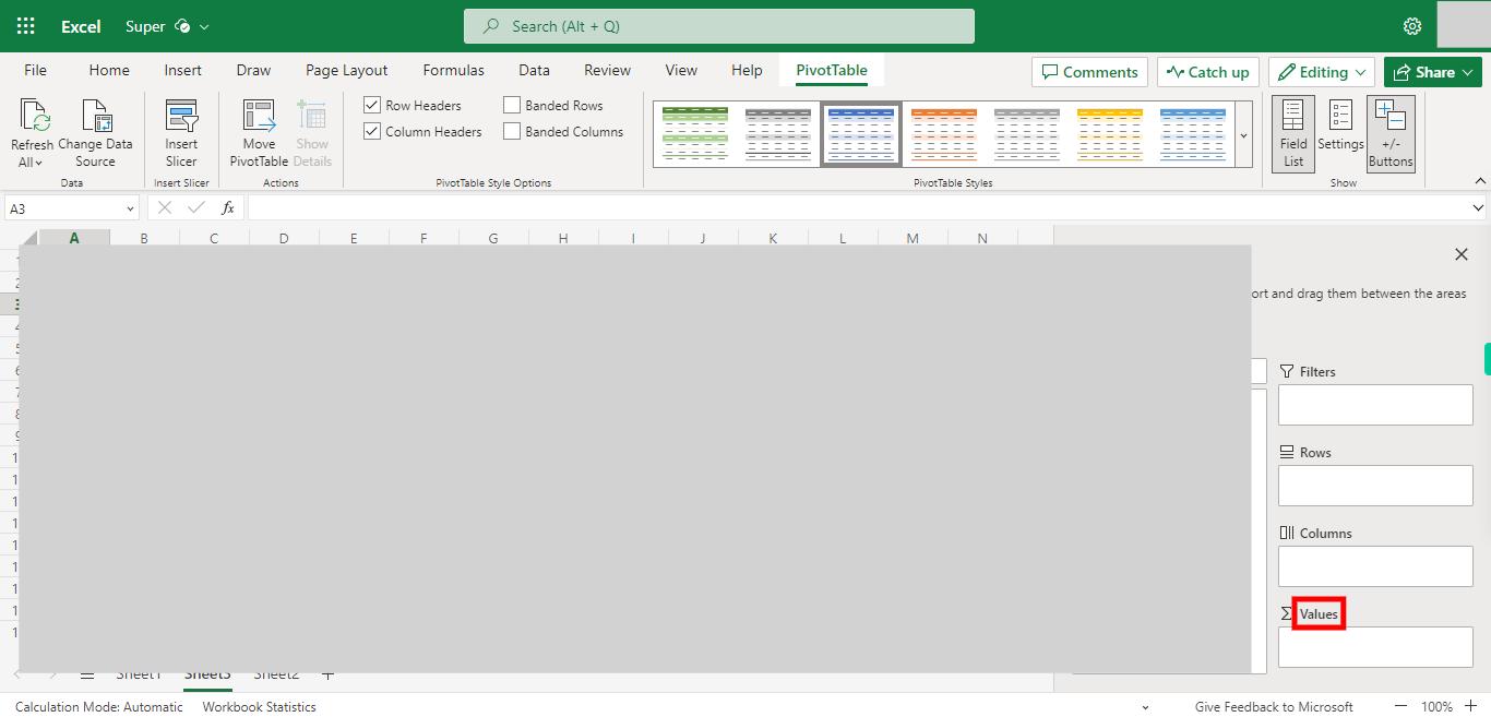
Drag and Drop the value you want to see in the Pivot. which will show the Count of values of a mentioned column. Once done, click on the "Close" button on the Supervity instruction widget.


