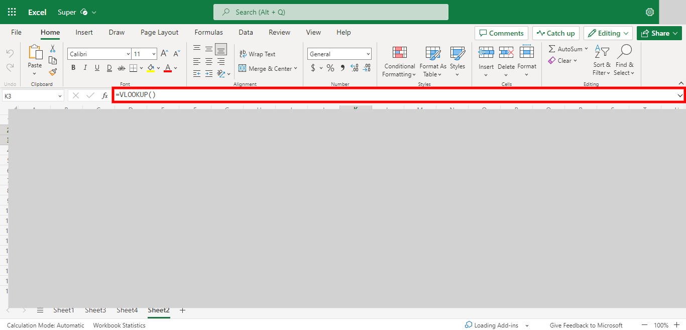
Step by step process of Adding a VLOOKUP formula for a cell to compare with the Whole column in the Different sheet. NOTE: to Use this Skill User needs to log in to Microsoft Applications.
-
1.
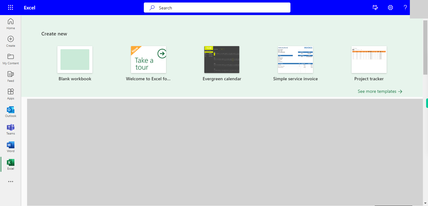
Open Microsoft Excel on the Web
-
2.
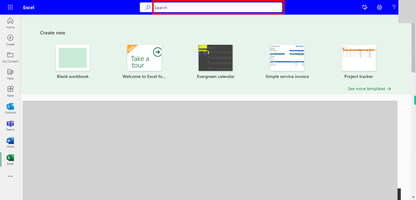
Click on Search Bar, Which enables the User to find the files in Outlook Excel. Type the file name, which will show recently Opened files. Once done, click on the "Next" button on the Supervity instruction widget. Open the File under the Search bar.
-
3.
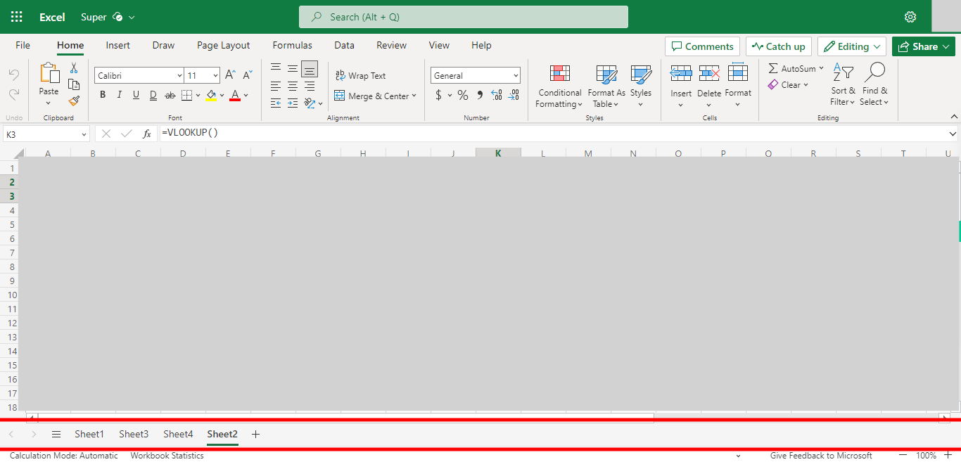
Go to the Sheet Where you want to Apply the VLookUp Formula for the Cell. Once done, click on the "Next" button on the Supervity instruction widget.
-
4.
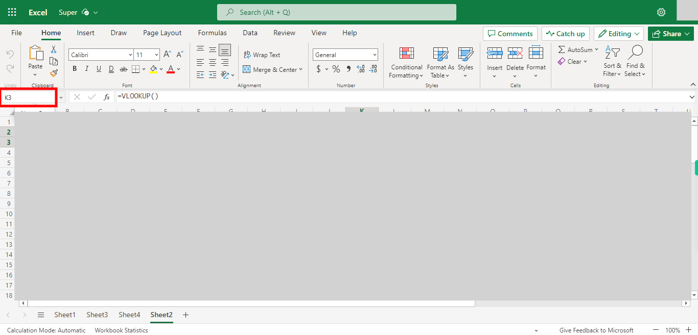
Click on Name Box, Enter the Cell Address, and click on Enter. Once done, click on the "Next" button on the Supervity instruction widget.
-
5.
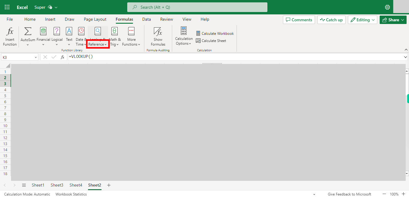
Click on Formulas Button.
-
6.
Click on Lookup & Reference dropdown.
-
7.
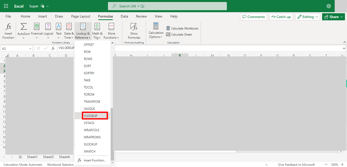
Click on VLOOKUP.
-
8.
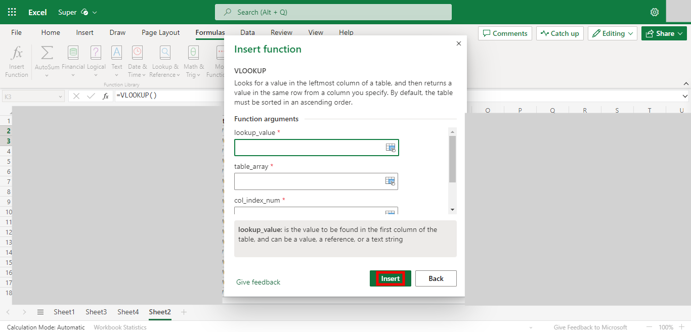
Click on Insert to add the VLOOKUP formula into that Cell.
-
9.
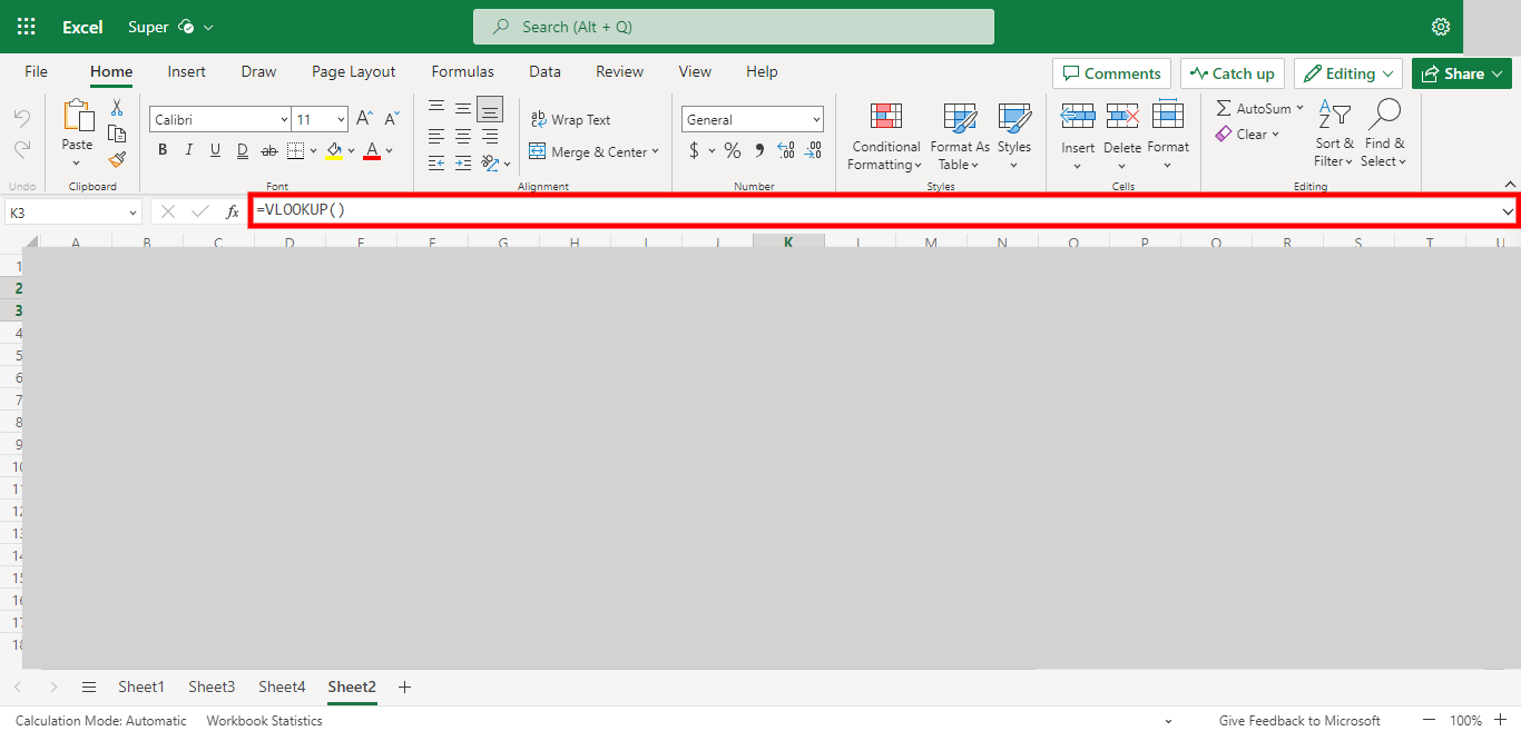
Add the Main Cell Address inside the VLOOKUP function eg: =VLOOKUP(H1, Once done, click on the "Next" button on the Supervity instruction widget.
-
10.
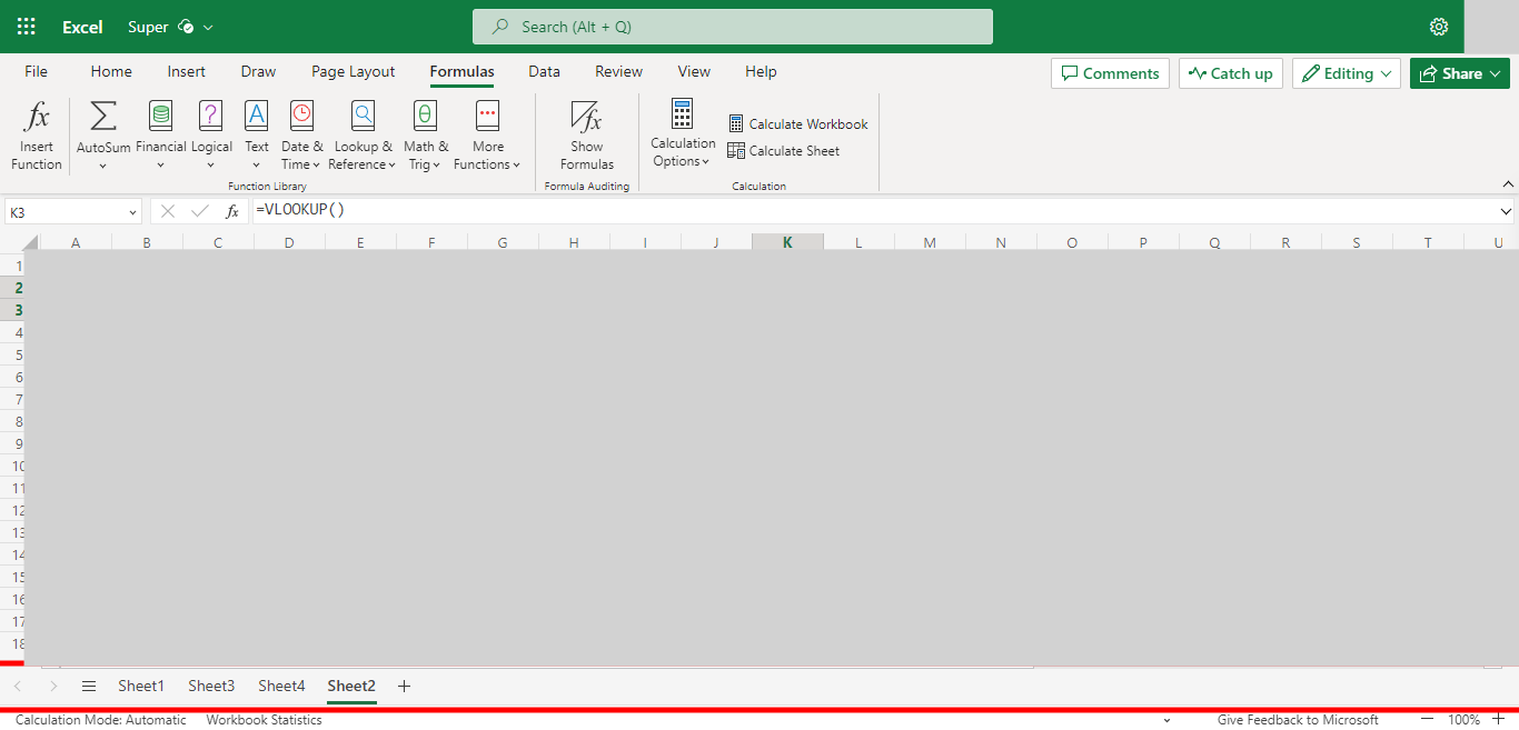
Go to the Sheet, Where you have the Column data to compare with. Once done, click on the "Next" button on the Supervity instruction widget.
-
11.
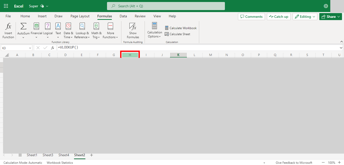
Click on the Column Address to select the whole column. Once done, click on the "Next" button on the Supervity instruction widget.
-
12.
Inside the Formula, the selected values will be reflected. Add the remaining condition in the formula as mentioned below. eg: " =VLOOKUP(H3,'Sheet4'!A:A,1,FALSE) " Once done, click on the "Close" button on the Supervity instruction widget.


